Tutorials

For deep learning, this tutorial will walk you through building handwritten digits classifiers using the MNIST dataset, arguably the “Hello World” of neural networks. For reinforcement learning, we will let computer learns to play Pong game from the original screen inputs. For nature language processing, we start from word embedding and then describe language modeling and machine translation.

This tutorial includes all modularized implementation of Google TensorFlow Deep Learning tutorial, so you could read TensorFlow Deep Learning tutorial at the same time [en] [cn] .

Note

For experts: Read the source code of InputLayer and DenseLayer, you will understand how TensorLayer work. After that, we recommend you to read the codes on Github directly.

Before we start

The tutorial assumes that you are somewhat familiar with neural networks and TensorFlow (the library which TensorLayer is built on top of). You can try to learn the basics of a neural network from the Deeplearning Tutorial.

For a more slow-paced introduction to artificial neural networks, we recommend Convolutional Neural Networks for Visual Recognition by Andrej Karpathy et al., Neural Networks and Deep Learning by Michael Nielsen.

To learn more about TensorFlow, have a look at the TensorFlow tutorial. You will not need all of it, but a basic understanding of how TensorFlow works is required to be able to use TensorLayer. If you’re new to TensorFlow, going through that tutorial.

TensorLayer is simple

The following code shows a simple example of TensorLayer, see tutorial_mnist_simple.py . We provide a lot of simple functions （like fit() , test() ), however, if you want to understand the details and be a machine learning expert, we suggest you to train the network by using the data iteration toolbox (tl.iterate) and the TensorFlow’s native API like sess.run(), see tutorial_mnist.py <https://github.com/tensorlayer/tensorlayer/blob/master/example/tutorial_mnist.py>_ , tutorial_mlp_dropout1.py and tutorial_mlp_dropout2.py <https://github.com/tensorlayer/tensorlayer/blob/master/example/tutorial_mlp_dropout2.py>_ for more details.

import tensorflow as tf
import tensorlayer as tl

sess = tf.InteractiveSession()

# prepare data
X_train, y_train, X_val, y_val, X_test, y_test = \
                                tl.files.load_mnist_dataset(shape=(-1,784))

# define placeholder
x = tf.placeholder(tf.float32, shape=[None, 784], name='x')
y_ = tf.placeholder(tf.int64, shape=[None, ], name='y_')

# define the network
network = tl.layers.InputLayer(x, name='input_layer')
network = tl.layers.DropoutLayer(network, keep=0.8, name='drop1')
network = tl.layers.DenseLayer(network, n_units=800,
                                act = tf.nn.relu, name='relu1')
network = tl.layers.DropoutLayer(network, keep=0.5, name='drop2')
network = tl.layers.DenseLayer(network, n_units=800,
                                act = tf.nn.relu, name='relu2')
network = tl.layers.DropoutLayer(network, keep=0.5, name='drop3')
# the softmax is implemented internally in tl.cost.cross_entropy(y, y_, 'cost') to
# speed up computation, so we use identity here.
# see tf.nn.sparse_softmax_cross_entropy_with_logits()
network = tl.layers.DenseLayer(network, n_units=10,
                                act = tf.identity,
                                name='output_layer')
# define cost function and metric.
y = network.outputs
cost = tl.cost.cross_entropy(y, y_, 'cost')
correct_prediction = tf.equal(tf.argmax(y, 1), y_)
acc = tf.reduce_mean(tf.cast(correct_prediction, tf.float32))
y_op = tf.argmax(tf.nn.softmax(y), 1)

# define the optimizer
train_params = network.all_params
train_op = tf.train.AdamOptimizer(learning_rate=0.0001, beta1=0.9, beta2=0.999,
                            epsilon=1e-08, use_locking=False).minimize(cost, var_list=train_params)

# initialize all variables in the session
tl.layers.initialize_global_variables(sess)

# print network information
network.print_params()
network.print_layers()

# train the network
tl.utils.fit(sess, network, train_op, cost, X_train, y_train, x, y_,
            acc=acc, batch_size=500, n_epoch=500, print_freq=5,
            X_val=X_val, y_val=y_val, eval_train=False)

# evaluation
tl.utils.test(sess, network, acc, X_test, y_test, x, y_, batch_size=None, cost=cost)

# save the network to .npz file
tl.files.save_npz(network.all_params , name='model.npz')
sess.close()

Run the MNIST example

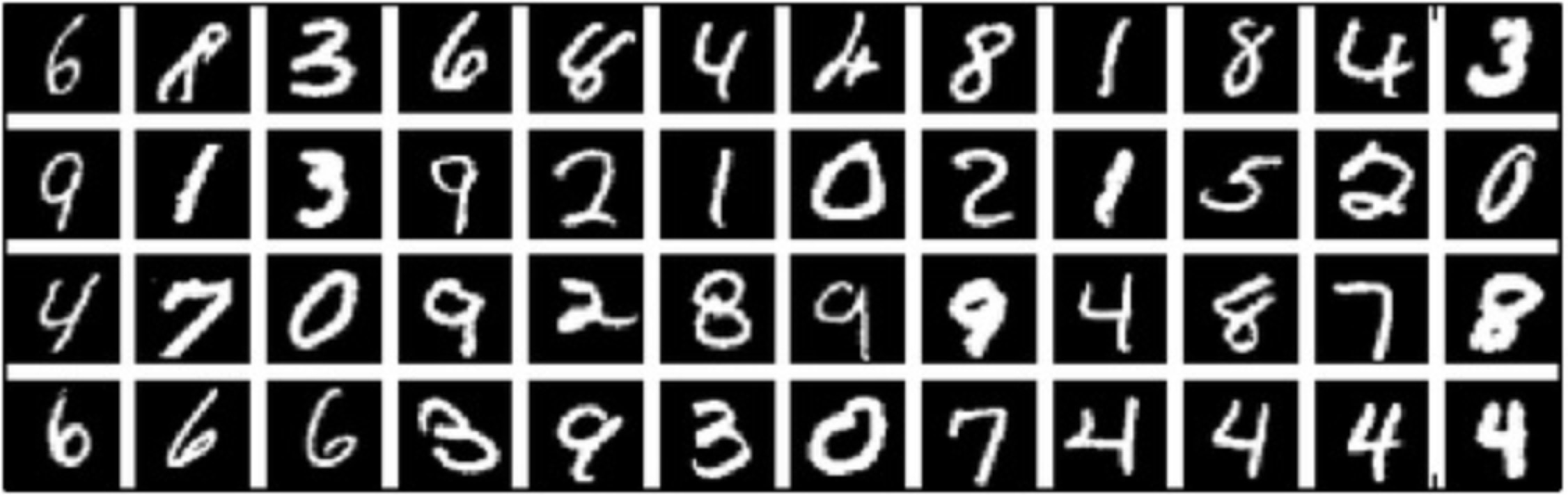
In the first part of the tutorial, we will just run the MNIST example that’s included in the source distribution of TensorLayer. The MNIST dataset contains 60000 handwritten digits that are commonly used for training various image processing systems. Each digit is 28x28 pixels in size.

We assume that you have already run through the Installation. If you haven’t done so already, get a copy of the source tree of TensorLayer, and navigate to the folder in a terminal window. Enter the folder and run the tutorial_mnist.py example script:

python tutorial_mnist.py

If everything is set up correctly, you will get an output like the following:

tensorlayer: GPU MEM Fraction 0.300000
Downloading train-images-idx3-ubyte.gz
Downloading train-labels-idx1-ubyte.gz
Downloading t10k-images-idx3-ubyte.gz
Downloading t10k-labels-idx1-ubyte.gz

X_train.shape (50000, 784)
y_train.shape (50000,)
X_val.shape (10000, 784)
y_val.shape (10000,)
X_test.shape (10000, 784)
y_test.shape (10000,)
X float32   y int64

[TL] InputLayer   input_layer (?, 784)
[TL] DropoutLayer drop1: keep: 0.800000
[TL] DenseLayer   relu1: 800, relu
[TL] DropoutLayer drop2: keep: 0.500000
[TL] DenseLayer   relu2: 800, relu
[TL] DropoutLayer drop3: keep: 0.500000
[TL] DenseLayer   output_layer: 10, identity

param 0: (784, 800) (mean: -0.000053, median: -0.000043 std: 0.035558)
param 1: (800,)     (mean:  0.000000, median:  0.000000 std: 0.000000)
param 2: (800, 800) (mean:  0.000008, median:  0.000041 std: 0.035371)
param 3: (800,)     (mean:  0.000000, median:  0.000000 std: 0.000000)
param 4: (800, 10)  (mean:  0.000469, median:  0.000432 std: 0.049895)
param 5: (10,)      (mean:  0.000000, median:  0.000000 std: 0.000000)
num of params: 1276810

layer 0: Tensor("dropout/mul_1:0", shape=(?, 784), dtype=float32)
layer 1: Tensor("Relu:0", shape=(?, 800), dtype=float32)
layer 2: Tensor("dropout_1/mul_1:0", shape=(?, 800), dtype=float32)
layer 3: Tensor("Relu_1:0", shape=(?, 800), dtype=float32)
layer 4: Tensor("dropout_2/mul_1:0", shape=(?, 800), dtype=float32)
layer 5: Tensor("add_2:0", shape=(?, 10), dtype=float32)

learning_rate: 0.000100
batch_size: 128

Epoch 1 of 500 took 0.342539s
  train loss: 0.330111
  val loss: 0.298098
  val acc: 0.910700
Epoch 10 of 500 took 0.356471s
  train loss: 0.085225
  val loss: 0.097082
  val acc: 0.971700
Epoch 20 of 500 took 0.352137s
  train loss: 0.040741
  val loss: 0.070149
  val acc: 0.978600
Epoch 30 of 500 took 0.350814s
  train loss: 0.022995
  val loss: 0.060471
  val acc: 0.982800
Epoch 40 of 500 took 0.350996s
  train loss: 0.013713
  val loss: 0.055777
  val acc: 0.983700
...

The example script allows you to try different models, including Multi-Layer Perceptron, Dropout, Dropconnect, Stacked Denoising Autoencoder and Convolutional Neural Network. Select different models from if __name__ == '__main__':.

main_test_layers(model='relu')
main_test_denoise_AE(model='relu')
main_test_stacked_denoise_AE(model='relu')
main_test_cnn_layer()

Understand the MNIST example

Let’s now investigate what’s needed to make that happen! To follow along, open up the source code.

Preface

The first thing you might notice is that besides TensorLayer, we also import numpy and tensorflow:

import tensorflow as tf
import tensorlayer as tl
from tensorlayer.layers import set_keep
import numpy as np
import time

As we know, TensorLayer is built on top of TensorFlow, it is meant as a supplement helping with some tasks, not as a replacement. You will always mix TensorLayer with some vanilla TensorFlow code. The set_keep is used to access the placeholder of keeping probabilities when using Denoising Autoencoder.

Loading data

The first piece of code defines a function load_mnist_dataset(). Its purpose is to download the MNIST dataset (if it hasn’t been downloaded yet) and return it in the form of regular numpy arrays. There is no TensorLayer involved at all, so for the purpose of this tutorial, we can regard it as:

X_train, y_train, X_val, y_val, X_test, y_test = \
                  tl.files.load_mnist_dataset(shape=(-1,784))

X_train.shape is (50000, 784), to be interpreted as: 50,000 images and each image has 784 pixels. y_train.shape is simply (50000,), which is a vector the same length of X_train giving an integer class label for each image – namely, the digit between 0 and 9 depicted in the image (according to the human annotator who drew that digit).

For Convolutional Neural Network example, the MNIST can be load as 4D version as follow:

X_train, y_train, X_val, y_val, X_test, y_test = \
            tl.files.load_mnist_dataset(shape=(-1, 28, 28, 1))

X_train.shape is (50000, 28, 28, 1) which represents 50,000 images with 1 channel, 28 rows and 28 columns each. Channel one is because it is a grey scale image, every pixel has only one value.

Building the model

This is where TensorLayer steps in. It allows you to define an arbitrarily structured neural network by creating and stacking or merging layers. Since every layer knows its immediate incoming layers, the output layer (or output layers) of a network double as a handle to the network as a whole, so usually this is the only thing we will pass on to the rest of the code.

As mentioned above, tutorial_mnist.py supports four types of models, and we implement that via easily exchangeable functions of the same interface. First, we’ll define a function that creates a Multi-Layer Perceptron (MLP) of a fixed architecture, explaining all the steps in detail. We’ll then implement a Denoising Autoencoder (DAE), after that we will then stack all Denoising Autoencoder and supervised fine-tune them. Finally, we’ll show how to create a Convolutional Neural Network (CNN). In addition, a simple example for MNIST dataset in tutorial_mnist_simple.py, a CNN example for the CIFAR-10 dataset in tutorial_cifar10_tfrecord.py.

Multi-Layer Perceptron (MLP)

The first script, main_test_layers(), creates an MLP of two hidden layers of 800 units each, followed by a softmax output layer of 10 units. It applies 20% dropout to the input data and 50% dropout to the hidden layers.

To feed data into the network, TensofFlow placeholders need to be defined as follow. The None here means the network will accept input data of arbitrary batch size after compilation. The x is used to hold the X_train data and y_ is used to hold the y_train data. If you know the batch size beforehand and do not need this flexibility, you should give the batch size here – especially for convolutional layers, this can allow TensorFlow to apply some optimizations.

x = tf.placeholder(tf.float32, shape=[None, 784], name='x')
y_ = tf.placeholder(tf.int64, shape=[None, ], name='y_')

The foundation of each neural network in TensorLayer is an InputLayer instance representing the input data that will subsequently be fed to the network. Note that the InputLayer is not tied to any specific data yet.

network = tl.layers.InputLayer(x, name='input')

Before adding the first hidden layer, we’ll apply 20% dropout to the input data. This is realized via a DropoutLayer instance:

network = tl.layers.DropoutLayer(network, keep=0.8, name='drop1')

Note that the first constructor argument is the incoming layer, the second argument is the keeping probability for the activation value. Now we’ll proceed with the first fully-connected hidden layer of 800 units. Note that when stacking a DenseLayer.

network = tl.layers.DenseLayer(network, n_units=800, act = tf.nn.relu, name='relu1')

Again, the first constructor argument means that we’re stacking network on top of network. n_units simply gives the number of units for this fully-connected layer. act takes an activation function, several of which are defined in tensorflow.nn and tensorlayer.activation. Here we’ve chosen the rectifier, so we’ll obtain ReLUs. We’ll now add dropout of 50%, another 800-unit dense layer and 50% dropout again:

network = tl.layers.DropoutLayer(network, keep=0.5, name='drop2')
network = tl.layers.DenseLayer(network, n_units=800, act = tf.nn.relu, name='relu2')
network = tl.layers.DropoutLayer(network, keep=0.5, name='drop3')

Finally, we’ll add the fully-connected output layer which the n_units equals to the number of classes. Note that, the softmax is implemented internally in tf.nn.sparse_softmax_cross_entropy_with_logits() to speed up computation, so we used identity in the last layer, more details in tl.cost.cross_entropy().

network = tl.layers.DenseLayer(network,
                              n_units=10,
                              act = tf.identity,
                              name='output')

As mentioned above, each layer is linked to its incoming layer(s), so we only need the output layer(s) to access a network in TensorLayer:

y = network.outputs
y_op = tf.argmax(tf.nn.softmax(y), 1)
cost = tf.reduce_mean(tf.nn.sparse_softmax_cross_entropy_with_logits(y, y_))

Here, network.outputs is the 10 identity outputs from the network (in one hot format), y_op is the integer output represents the class index. While cost is the cross-entropy between the target and the predicted labels.

Denoising Autoencoder (DAE)

Autoencoder is an unsupervised learning model which is able to extract representative features, it has become more widely used for learning generative models of data and Greedy layer-wise pre-train. For vanilla Autoencoder, see Deeplearning Tutorial.

The script main_test_denoise_AE() implements a Denoising Autoencoder with corrosion rate of 50%. The Autoencoder can be defined as follow, where an Autoencoder is represented by a DenseLayer:

network = tl.layers.InputLayer(x, name='input_layer')
network = tl.layers.DropoutLayer(network, keep=0.5, name='denoising1')
network = tl.layers.DenseLayer(network, n_units=200, act=tf.nn.sigmoid, name='sigmoid1')
recon_layer1 = tl.layers.ReconLayer(network,
                                    x_recon=x,
                                    n_units=784,
                                    act=tf.nn.sigmoid,
                                    name='recon_layer1')

To train the DenseLayer, simply run ReconLayer.pretrain(), if using denoising Autoencoder, the name of corrosion layer (a DropoutLayer) need to be specified as follow. To save the feature images, set save to True. There are many kinds of pre-train metrices according to different architectures and applications. For sigmoid activation, the Autoencoder can be implemented by using KL divergence, while for rectifier, L1 regularization of activation outputs can make the output to be sparse. So the default behaviour of ReconLayer only provide KLD and cross-entropy for sigmoid activation function and L1 of activation outputs and mean-squared-error for rectifying activation function. We recommend you to modify ReconLayer to achieve your own pre-train metrice.

recon_layer1.pretrain(sess,
                      x=x,
                      X_train=X_train,
                      X_val=X_val,
                      denoise_name='denoising1',
                      n_epoch=200,
                      batch_size=128,
                      print_freq=10,
                      save=True,
                      save_name='w1pre_')

In addition, the script main_test_stacked_denoise_AE() shows how to stacked multiple Autoencoder to one network and then fine-tune.

Convolutional Neural Network (CNN)

Finally, the main_test_cnn_layer() script creates two CNN layers and max pooling stages, a fully-connected hidden layer and a fully-connected output layer. More CNN examples can be found in other examples, like tutorial_cifar10_tfrecord.py.

network = tl.layers.Conv2d(network, 32, (5, 5), (1, 1),
        act=tf.nn.relu, padding='SAME', name='cnn1')
network = tl.layers.MaxPool2d(network, (2, 2), (2, 2),
        padding='SAME', name='pool1')
network = tl.layers.Conv2d(network, 64, (5, 5), (1, 1),
        act=tf.nn.relu, padding='SAME', name='cnn2')
network = tl.layers.MaxPool2d(network, (2, 2), (2, 2),
        padding='SAME', name='pool2')

network = tl.layers.FlattenLayer(network, name='flatten')
network = tl.layers.DropoutLayer(network, keep=0.5, name='drop1')
network = tl.layers.DenseLayer(network, 256, act=tf.nn.relu, name='relu1')
network = tl.layers.DropoutLayer(network, keep=0.5, name='drop2')
network = tl.layers.DenseLayer(network, 10, act=tf.identity, name='output')

Training the model

The remaining part of the tutorial_mnist.py script copes with setting up and running a training loop over the MNIST dataset by using cross-entropy only.

Dataset iteration

An iteration function for synchronously iterating over two numpy arrays of input data and targets, respectively, in mini-batches of a given number of items. More iteration function can be found in tensorlayer.iterate

tl.iterate.minibatches(inputs, targets, batchsize, shuffle=False)

Loss and update expressions

Continuing, we create a loss expression to be minimized in training:

y = network.outputs
y_op = tf.argmax(tf.nn.softmax(y), 1)
cost = tf.reduce_mean(tf.nn.sparse_softmax_cross_entropy_with_logits(y, y_))

More cost or regularization can be applied here. For example, to apply max-norm on the weight matrices, we can add the following line.

cost = cost + tl.cost.maxnorm_regularizer(1.0)(network.all_params[0]) +
              tl.cost.maxnorm_regularizer(1.0)(network.all_params[2])

Depending on the problem you are solving, you will need different loss functions, see tensorlayer.cost for more. Apart from using network.all_params to get the variables, we can also use tl.layers.get_variables_with_name to get the specific variables by string name.

Having the model and the loss function here, we create update expression/operation for training the network. TensorLayer does not provide many optimizers, we used TensorFlow’s optimizer instead:

train_params = network.all_params
train_op = tf.train.AdamOptimizer(learning_rate, beta1=0.9, beta2=0.999,
    epsilon=1e-08, use_locking=False).minimize(cost, var_list=train_params)

For training the network, we fed data and the keeping probabilities to the feed_dict.

feed_dict = {x: X_train_a, y_: y_train_a}
feed_dict.update( network.all_drop )
sess.run(train_op, feed_dict=feed_dict)

While, for validation and testing, we use slightly different way. All Dropout, Dropconnect, Corrosion layers need to be disabled. We use tl.utils.dict_to_one to set all network.all_drop to 1.

dp_dict = tl.utils.dict_to_one( network.all_drop )
feed_dict = {x: X_test_a, y_: y_test_a}
feed_dict.update(dp_dict)
err, ac = sess.run([cost, acc], feed_dict=feed_dict)

For evaluation, we create an expression for the classification accuracy:

correct_prediction = tf.equal(tf.argmax(y, 1), y_)
acc = tf.reduce_mean(tf.cast(correct_prediction, tf.float32))

What Next?

We also have a more advanced image classification example in tutorial_cifar10_tfrecord.py. Please read the code and notes, figure out how to generate more training data and what is local response normalization. After that, try to implement Residual Network (Hint: you may want to use the Layer.outputs).

Run the Pong Game example

In the second part of the tutorial, we will run the Deep Reinforcement Learning example which is introduced by Karpathy in Deep Reinforcement Learning: Pong from Pixels.

python tutorial_atari_pong.py

Before running the tutorial code, you need to install OpenAI gym environment which is a popular benchmark for Reinforcement Learning. If everything is set up correctly, you will get an output like the following:

[2016-07-12 09:31:59,760] Making new env: Pong-v0
  [TL] InputLayer input_layer (?, 6400)
  [TL] DenseLayer relu1: 200, relu
  [TL] DenseLayer output_layer: 3, identity
  param 0: (6400, 200) (mean: -0.000009  median: -0.000018 std: 0.017393)
  param 1: (200,)      (mean: 0.000000   median: 0.000000  std: 0.000000)
  param 2: (200, 3)    (mean: 0.002239   median: 0.003122  std: 0.096611)
  param 3: (3,)        (mean: 0.000000   median: 0.000000  std: 0.000000)
  num of params: 1280803
  layer 0: Tensor("Relu:0", shape=(?, 200), dtype=float32)
  layer 1: Tensor("add_1:0", shape=(?, 3), dtype=float32)
episode 0: game 0 took 0.17381s, reward: -1.000000
episode 0: game 1 took 0.12629s, reward: 1.000000  !!!!!!!!
episode 0: game 2 took 0.17082s, reward: -1.000000
episode 0: game 3 took 0.08944s, reward: -1.000000
episode 0: game 4 took 0.09446s, reward: -1.000000
episode 0: game 5 took 0.09440s, reward: -1.000000
episode 0: game 6 took 0.32798s, reward: -1.000000
episode 0: game 7 took 0.74437s, reward: -1.000000
episode 0: game 8 took 0.43013s, reward: -1.000000
episode 0: game 9 took 0.42496s, reward: -1.000000
episode 0: game 10 took 0.37128s, reward: -1.000000
episode 0: game 11 took 0.08979s, reward: -1.000000
episode 0: game 12 took 0.09138s, reward: -1.000000
episode 0: game 13 took 0.09142s, reward: -1.000000
episode 0: game 14 took 0.09639s, reward: -1.000000
episode 0: game 15 took 0.09852s, reward: -1.000000
episode 0: game 16 took 0.09984s, reward: -1.000000
episode 0: game 17 took 0.09575s, reward: -1.000000
episode 0: game 18 took 0.09416s, reward: -1.000000
episode 0: game 19 took 0.08674s, reward: -1.000000
episode 0: game 20 took 0.09628s, reward: -1.000000
resetting env. episode reward total was -20.000000. running mean: -20.000000
episode 1: game 0 took 0.09910s, reward: -1.000000
episode 1: game 1 took 0.17056s, reward: -1.000000
episode 1: game 2 took 0.09306s, reward: -1.000000
episode 1: game 3 took 0.09556s, reward: -1.000000
episode 1: game 4 took 0.12520s, reward: 1.000000  !!!!!!!!
episode 1: game 5 took 0.17348s, reward: -1.000000
episode 1: game 6 took 0.09415s, reward: -1.000000

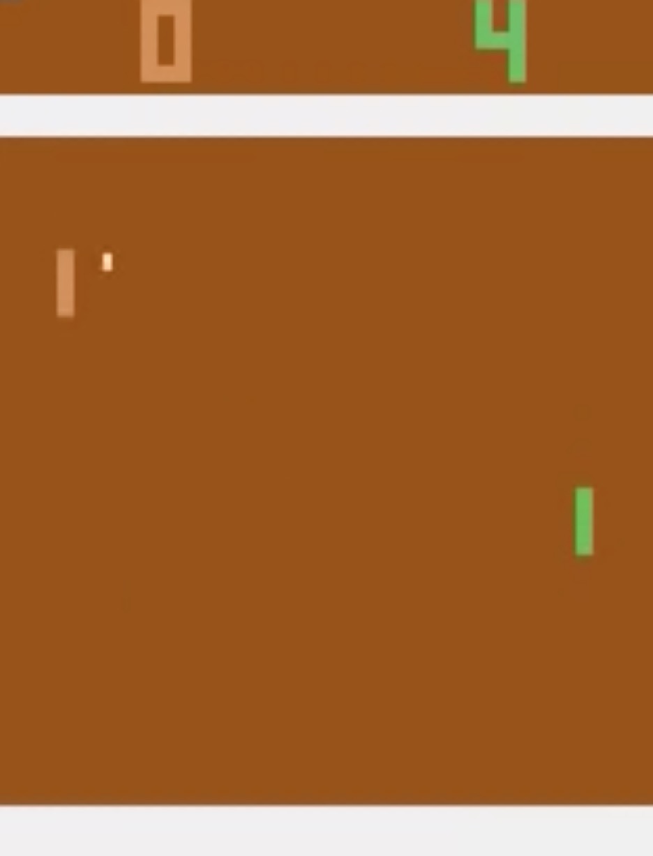
This example allows the neural network to learn how to play Pong game from the screen inputs, just like human behavior. The neural network will play with a fake AI player and learn to beat it. After training for 15,000 episodes, the neural network can win 20% of the games. The neural network win 35% of the games at 20,000 episode, we can seen the neural network learn faster and faster as it has more winning data to train. If you run it for 30,000 episode, it never loss.

render = False
resume = False

Setting render to True, if you want to display the game environment. When you run the code again, you can set resume to True, the code will load the existing model and train the model basic on it.

Understand Reinforcement learning

Pong Game

To understand Reinforcement Learning, we let computer to learn how to play Pong game from the original screen inputs. Before we start, we highly recommend you to go through a famous blog called Deep Reinforcement Learning: Pong from Pixels which is a minimalistic implementation of Deep Reinforcement Learning by using python-numpy and OpenAI gym environment.

python tutorial_atari_pong.py

Policy Network

In Deep Reinforcement Learning, the Policy Network is the same with Deep Neural Network, it is our player (or “agent”) who output actions to tell what we should do (move UP or DOWN); in Karpathy’s code, he only defined 2 actions, UP and DOWN and using a single simgoid output; In order to make our tutorial more generic, we defined 3 actions which are UP, DOWN and STOP (do nothing) by using 3 softmax outputs.

# observation for training
states_batch_pl = tf.placeholder(tf.float32, shape=[None, D])

network = tl.layers.InputLayer(states_batch_pl, name='input_layer')
network = tl.layers.DenseLayer(network, n_units=H,
                                act = tf.nn.relu, name='relu1')
network = tl.layers.DenseLayer(network, n_units=3,
                        act = tf.identity, name='output_layer')
probs = network.outputs
sampling_prob = tf.nn.softmax(probs)

Then when our agent is playing Pong, it calculates the probabilities of different actions, and then draw sample (action) from this uniform distribution. As the actions are represented by 1, 2 and 3, but the softmax outputs should be start from 0, we calculate the label value by minus 1.

prob = sess.run(
    sampling_prob,
    feed_dict={states_batch_pl: x}
)
# action. 1: STOP  2: UP  3: DOWN
action = np.random.choice([1,2,3], p=prob.flatten())
...
ys.append(action - 1)

Policy Gradient

Policy gradient methods are end-to-end algorithms that directly learn policy functions mapping states to actions. An approximate policy could be learned directly by maximizing the expected rewards. The parameters of a policy function (e.g. the parameters of a policy network used in the pong example) could be trained and learned under the guidance of the gradient of expected rewards. In other words, we can gradually tune the policy function via updating its parameters, such that it will generate actions from given states towards higher rewards.

An alternative method to policy gradient is Deep Q-Learning (DQN). It is based on Q-Learning that tries to learn a value function (called Q function) mapping states and actions to some value. DQN employs a deep neural network to represent the Q function as a function approximator. The training is done by minimizing temporal-difference errors. A neurobiologically inspired mechanism called “experience replay” is typically used along with DQN to help improve its stability caused by the use of non-linear function approximator.

You can check the following papers to gain better understandings about Reinforcement Learning.

• Reinforcement Learning: An Introduction. Richard S. Sutton and Andrew G. Barto
• Deep Reinforcement Learning. David Silver, Google DeepMind
• UCL Course on RL

The most successful applications of Deep Reinforcement Learning in recent years include DQN with experience replay to play Atari games and AlphaGO that for the first time beats world-class professional GO players. AlphaGO used the policy gradient method to train its policy network that is similar to the example of Pong game.

• Atari - Playing Atari with Deep Reinforcement Learning
• Atari - Human-level control through deep reinforcement learning
• AlphaGO - Mastering the game of Go with deep neural networks and tree search

Dataset iteration

In Reinforcement Learning, we consider a final decision as an episode. In Pong game, a episode is a few dozen games, because the games go up to score of 21 for either player. Then the batch size is how many episode we consider to update the model. In the tutorial, we train a 2-layer policy network with 200 hidden layer units using RMSProp on batches of 10 episodes.

Loss and update expressions

We create a loss expression to be minimized in training:

actions_batch_pl = tf.placeholder(tf.int32, shape=[None])
discount_rewards_batch_pl = tf.placeholder(tf.float32, shape=[None])
loss = tl.rein.cross_entropy_reward_loss(probs, actions_batch_pl,
                                              discount_rewards_batch_pl)
...
...
sess.run(
    train_op,
    feed_dict={
        states_batch_pl: epx,
        actions_batch_pl: epy,
        discount_rewards_batch_pl: disR
    }
)

The loss in a batch is relate to all outputs of Policy Network, all actions we made and the corresponding discounted rewards in a batch. We first compute the loss of each action by multiplying the discounted reward and the cross-entropy between its output and its true action. The final loss in a batch is the sum of all loss of the actions.

What Next?

The tutorial above shows how you can build your own agent, end-to-end. While it has reasonable quality, the default parameters will not give you the best agent model. Here are a few things you can improve.

First of all, instead of conventional MLP model, we can use CNNs to capture the screen information better as Playing Atari with Deep Reinforcement Learning describe.

Also, the default parameters of the model are not tuned. You can try changing the learning rate, decay, or initializing the weights of your model in a different way.

Finally, you can try the model on different tasks (games) and try other reinforcement learning algorithm in Example.

Run the Word2Vec example

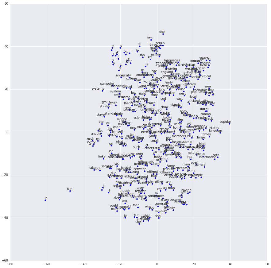
In this part of the tutorial, we train a matrix for words, where each word can be represented by a unique row vector in the matrix. In the end, similar words will have similar vectors. Then as we plot out the words into a two-dimensional plane, words that are similar end up clustering nearby each other.

python tutorial_word2vec_basic.py

If everything is set up correctly, you will get an output in the end.

Understand Word Embedding

Word Embedding

We highly recommend you to read Colah’s blog Word Representations to understand why we want to use a vector representation, and how to compute the vectors. (For chinese reader please click. More details about word2vec can be found in Word2vec Parameter Learning Explained.

Bascially, training an embedding matrix is an unsupervised learning. As every word is refected by an unique ID, which is the row index of the embedding matrix, a word can be converted into a vector, it can better represent the meaning. For example, there seems to be a constant male-female difference vector: woman − man = queen - king, this means one dimension in the vector represents gender.

The model can be created as follow.

# train_inputs is a row vector, a input is an integer id of single word.
# train_labels is a column vector, a label is an integer id of single word.
# valid_dataset is a column vector, a valid set is an integer id of single word.
train_inputs = tf.placeholder(tf.int32, shape=[batch_size])
train_labels = tf.placeholder(tf.int32, shape=[batch_size, 1])
valid_dataset = tf.constant(valid_examples, dtype=tf.int32)

# Look up embeddings for inputs.
emb_net = tl.layers.Word2vecEmbeddingInputlayer(
        inputs = train_inputs,
        train_labels = train_labels,
        vocabulary_size = vocabulary_size,
        embedding_size = embedding_size,
        num_sampled = num_sampled,
        nce_loss_args = {},
        E_init = tf.random_uniform_initializer(minval=-1.0, maxval=1.0),
        E_init_args = {},
        nce_W_init = tf.truncated_normal_initializer(
                          stddev=float(1.0/np.sqrt(embedding_size))),
        nce_W_init_args = {},
        nce_b_init = tf.constant_initializer(value=0.0),
        nce_b_init_args = {},
        name ='word2vec_layer',
    )

Dataset iteration and loss

Word2vec uses Negative Sampling and Skip-Gram model for training. Noise-Contrastive Estimation Loss (NCE) can help to reduce the computation of loss. Skip-Gram inverts context and targets, tries to predict each context word from its target word. We use tl.nlp.generate_skip_gram_batch to generate training data as follow, see tutorial_generate_text.py .

# NCE cost expression is provided by Word2vecEmbeddingInputlayer
cost = emb_net.nce_cost
train_params = emb_net.all_params

train_op = tf.train.AdagradOptimizer(learning_rate, initial_accumulator_value=0.1,
          use_locking=False).minimize(cost, var_list=train_params)

data_index = 0
while (step < num_steps):
  batch_inputs, batch_labels, data_index = tl.nlp.generate_skip_gram_batch(
                data=data, batch_size=batch_size, num_skips=num_skips,
                skip_window=skip_window, data_index=data_index)
  feed_dict = {train_inputs : batch_inputs, train_labels : batch_labels}
  _, loss_val = sess.run([train_op, cost], feed_dict=feed_dict)

Restore existing Embedding matrix

In the end of training the embedding matrix, we save the matrix and corresponding dictionaries. Then next time, we can restore the matrix and directories as follow. (see main_restore_embedding_layer() in tutorial_generate_text.py)

vocabulary_size = 50000
embedding_size = 128
model_file_name = "model_word2vec_50k_128"
batch_size = None

print("Load existing embedding matrix and dictionaries")
all_var = tl.files.load_npy_to_any(name=model_file_name+'.npy')
data = all_var['data']; count = all_var['count']
dictionary = all_var['dictionary']
reverse_dictionary = all_var['reverse_dictionary']

tl.nlp.save_vocab(count, name='vocab_'+model_file_name+'.txt')

del all_var, data, count

load_params = tl.files.load_npz(name=model_file_name+'.npz')

x = tf.placeholder(tf.int32, shape=[batch_size])
y_ = tf.placeholder(tf.int32, shape=[batch_size, 1])

emb_net = tl.layers.EmbeddingInputlayer(
                inputs = x,
                vocabulary_size = vocabulary_size,
                embedding_size = embedding_size,
                name ='embedding_layer')

tl.layers.initialize_global_variables(sess)

tl.files.assign_params(sess, [load_params[0]], emb_net)

Run the PTB example

Penn TreeBank (PTB) dataset is used in many LANGUAGE MODELING papers, including “Empirical Evaluation and Combination of Advanced Language Modeling Techniques”, “Recurrent Neural Network Regularization”. It consists of 929k training words, 73k validation words, and 82k test words. It has 10k words in its vocabulary.

The PTB example is trying to show how to train a recurrent neural network on a challenging task of language modeling.

Given a sentence “I am from Imperial College London”, the model can learn to predict “Imperial College London” from “from Imperial College”. In other word, it predict the next word in a text given a history of previous words. In the previous example , num_steps (sequence length) is 3.

python tutorial_ptb_lstm.py

The script provides three settings (small, medium, large), where a larger model has better performance. You can choose different settings in:

flags.DEFINE_string(
    "model", "small",
    "A type of model. Possible options are: small, medium, large.")

If you choose the small setting, you can see:

Epoch: 1 Learning rate: 1.000
0.004 perplexity: 5220.213 speed: 7635 wps
0.104 perplexity: 828.871 speed: 8469 wps
0.204 perplexity: 614.071 speed: 8839 wps
0.304 perplexity: 495.485 speed: 8889 wps
0.404 perplexity: 427.381 speed: 8940 wps
0.504 perplexity: 383.063 speed: 8920 wps
0.604 perplexity: 345.135 speed: 8920 wps
0.703 perplexity: 319.263 speed: 8949 wps
0.803 perplexity: 298.774 speed: 8975 wps
0.903 perplexity: 279.817 speed: 8986 wps
Epoch: 1 Train Perplexity: 265.558
Epoch: 1 Valid Perplexity: 178.436
...
Epoch: 13 Learning rate: 0.004
0.004 perplexity: 56.122 speed: 8594 wps
0.104 perplexity: 40.793 speed: 9186 wps
0.204 perplexity: 44.527 speed: 9117 wps
0.304 perplexity: 42.668 speed: 9214 wps
0.404 perplexity: 41.943 speed: 9269 wps
0.504 perplexity: 41.286 speed: 9271 wps
0.604 perplexity: 39.989 speed: 9244 wps
0.703 perplexity: 39.403 speed: 9236 wps
0.803 perplexity: 38.742 speed: 9229 wps
0.903 perplexity: 37.430 speed: 9240 wps
Epoch: 13 Train Perplexity: 36.643
Epoch: 13 Valid Perplexity: 121.475
Test Perplexity: 116.716

The PTB example shows that RNN is able to model language, but this example did not do something practically interesting. However, you should read through this example and “Understand LSTM” in order to understand the basics of RNN. After that, you will learn how to generate text, how to achieve language translation, and how to build a question answering system by using RNN.

Understand LSTM

Recurrent Neural Network

We personally think Andrej Karpathy’s blog is the best material to Understand Recurrent Neural Network , after reading that, Colah’s blog can help you to Understand LSTM Network [chinese] which can solve The Problem of Long-Term Dependencies. We will not describe more about the theory of RNN, so please read through these blogs before you go on.

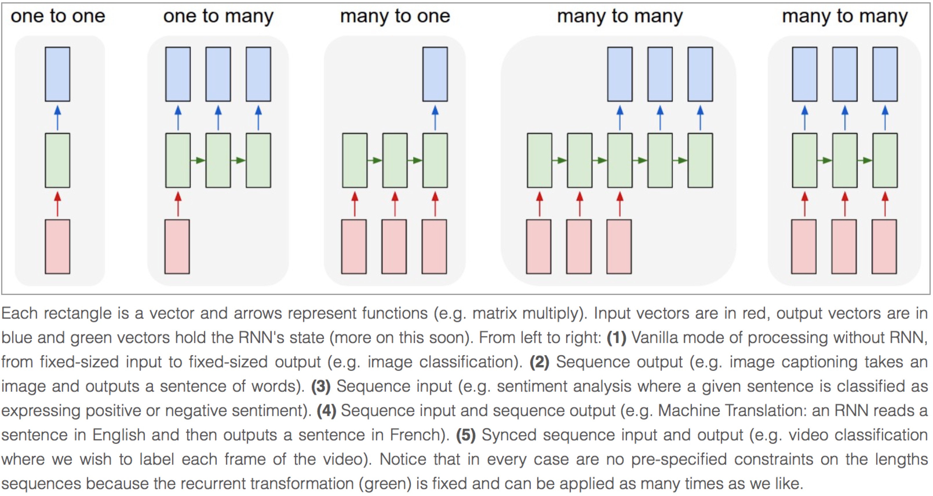
Image by Andrej Karpathy

Synced sequence input and output

The model in PTB example is a typical type of synced sequence input and output, which was described by Karpathy as “(5) Synced sequence input and output (e.g. video classification where we wish to label each frame of the video). Notice that in every case there are no pre-specified constraints on the lengths of sequences because the recurrent transformation (green) can be applied as many times as we like.”

The model is built as follows. Firstly, we transfer the words into word vectors by looking up an embedding matrix. In this tutorial, there is no pre-training on the embedding matrix. Secondly, we stack two LSTMs together using dropout between the embedding layer, LSTM layers, and the output layer for regularization. In the final layer, the model provides a sequence of softmax outputs.

The first LSTM layer outputs [batch_size, num_steps, hidden_size] for stacking another LSTM after it. The second LSTM layer outputs [batch_size*num_steps, hidden_size] for stacking a DenseLayer after it. Then the DenseLayer computes the softmax outputs of each example （n_examples = batch_size*num_steps).

To understand the PTB tutorial, you can also read TensorFlow PTB tutorial.

(Note that, TensorLayer supports DynamicRNNLayer after v1.1, so you can set the input/output dropouts, number of RNN layers in one single layer)

network = tl.layers.EmbeddingInputlayer(
            inputs = x,
            vocabulary_size = vocab_size,
            embedding_size = hidden_size,
            E_init = tf.random_uniform_initializer(-init_scale, init_scale),
            name ='embedding_layer')
if is_training:
    network = tl.layers.DropoutLayer(network, keep=keep_prob, name='drop1')
network = tl.layers.RNNLayer(network,
            cell_fn=tf.contrib.rnn.BasicLSTMCell,
            cell_init_args={'forget_bias': 0.0},
            n_hidden=hidden_size,
            initializer=tf.random_uniform_initializer(-init_scale, init_scale),
            n_steps=num_steps,
            return_last=False,
            name='basic_lstm_layer1')
lstm1 = network
if is_training:
    network = tl.layers.DropoutLayer(network, keep=keep_prob, name='drop2')
network = tl.layers.RNNLayer(network,
            cell_fn=tf.contrib.rnn.BasicLSTMCell,
            cell_init_args={'forget_bias': 0.0},
            n_hidden=hidden_size,
            initializer=tf.random_uniform_initializer(-init_scale, init_scale),
            n_steps=num_steps,
            return_last=False,
            return_seq_2d=True,
            name='basic_lstm_layer2')
lstm2 = network
if is_training:
    network = tl.layers.DropoutLayer(network, keep=keep_prob, name='drop3')
network = tl.layers.DenseLayer(network,
            n_units=vocab_size,
            W_init=tf.random_uniform_initializer(-init_scale, init_scale),
            b_init=tf.random_uniform_initializer(-init_scale, init_scale),
            act = tf.identity, name='output_layer')

Dataset iteration

The batch_size can be seen as the number of concurrent computations we are running. As the following example shows, the first batch learns the sequence information by using items 0 to 9. The second batch learn the sequence information by using items 10 to 19. So it ignores the information from items 9 to 10 !n If only if we set batch_size = 1`, it will consider all the information from items 0 to 20.

The meaning of batch_size here is not the same as the batch_size in the MNIST example. In the MNIST example, batch_size reflects how many examples we consider in each iteration, while in the PTB example, batch_size is the number of concurrent processes (segments) for accelerating the computation.

Some information will be ignored if batch_size > 1, however, if your dataset is “long” enough (a text corpus usually has billions of words), the ignored information would not affect the final result.

In the PTB tutorial, we set batch_size = 20, so we divide the dataset into 20 segments. At the beginning of each epoch, we initialize (reset) the 20 RNN states for the 20 segments to zero, then go through the 20 segments separately.

An example of generating training data is as follows:

train_data = [i for i in range(20)]
for batch in tl.iterate.ptb_iterator(train_data, batch_size=2, num_steps=3):
    x, y = batch
    print(x, '\n',y)

... [[ 0  1  2] <---x                       1st subset/ iteration
...  [10 11 12]]
... [[ 1  2  3] <---y
...  [11 12 13]]
...
... [[ 3  4  5]  <--- 1st batch input       2nd subset/ iteration
...  [13 14 15]] <--- 2nd batch input
... [[ 4  5  6]  <--- 1st batch target
...  [14 15 16]] <--- 2nd batch target
...
... [[ 6  7  8]                             3rd subset/ iteration
...  [16 17 18]]
... [[ 7  8  9]
...  [17 18 19]]

Note

This example can also be considered as pre-training of the word embedding matrix.

Loss and update expressions

The cost function is the average cost of each mini-batch:

# See tensorlayer.cost.cross_entropy_seq() for more details
def loss_fn(outputs, targets, batch_size, num_steps):
    # Returns the cost function of Cross-entropy of two sequences, implement
    # softmax internally.
    # outputs : 2D tensor [batch_size*num_steps, n_units of output layer]
    # targets : 2D tensor [batch_size, num_steps], need to be reshaped.
    # n_examples = batch_size * num_steps
    # so
    # cost is the average cost of each mini-batch (concurrent process).
    loss = tf.nn.seq2seq.sequence_loss_by_example(
        [outputs],
        [tf.reshape(targets, [-1])],
        [tf.ones([batch_size * num_steps])])
    cost = tf.reduce_sum(loss) / batch_size
    return cost

# Cost for Training
cost = loss_fn(network.outputs, targets, batch_size, num_steps)

For updating, truncated backpropagation clips values of gradients by the ratio of the sum of their norms, so as to make the learning process tractable.

# Truncated Backpropagation for training
with tf.variable_scope('learning_rate'):
    lr = tf.Variable(0.0, trainable=False)
tvars = tf.trainable_variables()
grads, _ = tf.clip_by_global_norm(tf.gradients(cost, tvars),
                                  max_grad_norm)
optimizer = tf.train.GradientDescentOptimizer(lr)
train_op = optimizer.apply_gradients(zip(grads, tvars))

In addition, if the epoch index is greater than max_epoch, we decrease the learning rate by multipling lr_decay.

new_lr_decay = lr_decay ** max(i - max_epoch, 0.0)
sess.run(tf.assign(lr, learning_rate * new_lr_decay))

At the beginning of each epoch, all states of LSTMs need to be reseted (initialized) to zero states. Then after each iteration, the LSTMs’ states is updated, so the new LSTM states (final states) need to be assigned as the initial states of the next iteration:

# set all states to zero states at the beginning of each epoch
state1 = tl.layers.initialize_rnn_state(lstm1.initial_state)
state2 = tl.layers.initialize_rnn_state(lstm2.initial_state)
for step, (x, y) in enumerate(tl.iterate.ptb_iterator(train_data,
                                            batch_size, num_steps)):
    feed_dict = {input_data: x, targets: y,
                lstm1.initial_state: state1,
                lstm2.initial_state: state2,
                }
    # For training, enable dropout
    feed_dict.update( network.all_drop )
    # use the new states as the initial state of next iteration
    _cost, state1, state2, _ = sess.run([cost,
                                    lstm1.final_state,
                                    lstm2.final_state,
                                    train_op],
                                    feed_dict=feed_dict
                                    )
    costs += _cost; iters += num_steps

Predicting

After training the model, when we predict the next output, we no long consider the number of steps (sequence length), i.e. batch_size, num_steps are set to 1. Then we can output the next word one by one, instead of predicting a sequence of words from a sequence of words.

input_data_test = tf.placeholder(tf.int32, [1, 1])
targets_test = tf.placeholder(tf.int32, [1, 1])
...
network_test, lstm1_test, lstm2_test = inference(input_data_test,
                      is_training=False, num_steps=1, reuse=True)
...
cost_test = loss_fn(network_test.outputs, targets_test, 1, 1)
...
print("Evaluation")
# Testing
# go through the test set step by step, it will take a while.
start_time = time.time()
costs = 0.0; iters = 0
# reset all states at the beginning
state1 = tl.layers.initialize_rnn_state(lstm1_test.initial_state)
state2 = tl.layers.initialize_rnn_state(lstm2_test.initial_state)
for step, (x, y) in enumerate(tl.iterate.ptb_iterator(test_data,
                                        batch_size=1, num_steps=1)):
    feed_dict = {input_data_test: x, targets_test: y,
                lstm1_test.initial_state: state1,
                lstm2_test.initial_state: state2,
                }
    _cost, state1, state2 = sess.run([cost_test,
                                    lstm1_test.final_state,
                                    lstm2_test.final_state],
                                    feed_dict=feed_dict
                                    )
    costs += _cost; iters += 1
test_perplexity = np.exp(costs / iters)
print("Test Perplexity: %.3f took %.2fs" % (test_perplexity, time.time() - start_time))

What Next?

Now, you have understood Synced sequence input and output. Let’s think about Many to one (Sequence input and one output), so that LSTM is able to predict the next word “English” from “I am from London, I speak ..”.

Please read and understand the code of tutorial_generate_text.py. It shows you how to restore a pre-trained Embedding matrix and how to learn text generation from a given context.

Karpathy’s blog : “(3) Sequence input (e.g. sentiment analysis where a given sentence is classified as expressing positive or negative sentiment). “

More Tutorials

In Example page, we provide many examples include Seq2seq, different type of Adversarial Learning, Reinforcement Learning and etc.

More info

For more information on what you can do with TensorLayer, just continue reading through readthedocs. Finally, the reference lists and explains as follow.

layers (tensorlayer.layers),

activation (tensorlayer.activation),

natural language processing (tensorlayer.nlp),

reinforcement learning (tensorlayer.rein),

cost expressions and regularizers (tensorlayer.cost),

load and save files (tensorlayer.files),

helper functions (tensorlayer.utils),

visualization (tensorlayer.visualize),

iteration functions (tensorlayer.iterate),

preprocessing functions (tensorlayer.prepro),

command line interface (tensorlayer.prepro),